RESAMPLING METHODS, PART I – JACKKNIFE METHODS

1. Validation Set Approach

> attach(Auto); n = length(mpg);

> Z = sample( n, n/2 ) # Random subsample of size n/2

# Works similarly to generating a Bernoulli variable

> reg.fit = lm( mpg ~ weight + horsepower + acceleration, subset=Z ) # Fit using training data

> mpg_predicted = predict( reg.fit, Auto )

# Use this model to predict the testing data [-Z]

> plot(mpg[-Z],mpg_predicted[-Z]) # We can see a nonlinear component

> abline(0,1) # Compare with the line y=x.

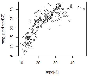
> mean( (mpg - mpg_predicted) [-Z]^2 ) # Estimate the mean-squared error MSE

[1] 20.46885

2. Jackknife (Leave-One-Out Cross-Validation, LOOCV)

> install.packages(“boot”)

> library(boot)

> glm.fit = glm(mpg ~ weight + horsepower + acceleration) # Default “family” is Normal, so this GLM model

> cv.error = cv.glm( Auto, glm.fit ) # is the same as LM, standard linear regression.

> names(cv.error) # This cross-validation tool has several outputs

[1] "call" "K" "delta" "seed" # We are interested in “delta”

> error$delta

[1] 18.25595 18.25542

# Delta consists of 2 numbers – estimated prediction error and its version adjusted for the lost sample size due to cross-validation.

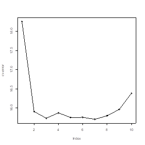
# Example – what power of “horsepower” is optimal for this prediction?

> cv.error = rep(0,10) # Initiate a vector of estimated errors

> for (p in 1:10){ # Fit polynomial regression models

+ glm.fit = glm( mpg ~ weight + poly(horsepower,p) + acceleration ) # with power p=1..10

+ cv.error[p] = cv.glm( Auto, glm.fit )$delta[1] } # Save prediction errors

> cv.error # Look at the results

[1] 18.25595 15.90163 15.72995 15.86879 15.74517 15.74989 15.70073 15.79314 15.95933 16.38301

# Although p=7 yields the lowest estimated prediction error, after p=2, the improvement is very little.

> plot(cv.error)

> lines(cv.error)

# Package “bootstrap” has a jackknife tool. For example, here is a bias reduction for a sample variance.

# We’ll start with the biased version of a sample variance (it’s MLE, under Normal distribution)

> variance.fn = function(X){ return( mean( (X-mean(X))^2 ) ) }

> variance.fn(mpg)

[1] 60.76274

# Use jackknife to correct its bias.

> install.packages(“bootstrap”)

> library(bootstrap)

> variance.JK = jackknife( mpg, variance.fn )

# This gives us the jackknife estimates of standard error and bias, as well as all estimates _(-i)

> variance.JK

$jack.se

[1] 3.741951

$jack.bias

[1] -0.1554034

$jack.values

[1] 60.84210 60.73524 60.84210 60.77598 60.81160 60.73524 60.68936 60.68936 60.68936 60.73524 60.73524 60.68936 60.73524 60.68936 60.91735 60.91278 60.84210 60.90280

[19] 60.88575 60.90142 60.91195 60.91735 60.91195 60.90142 60.90280 60.45457 60.45457 60.52096 60.38306 60.88575 60.86496 60.91195 60.86746 60.77598 60.81160 60.86746

[37] 60.84210 60.68936 60.68936 60.68936 60.68936 60.58222 60.63836 60.63836 60.84210 60.91278 60.86746 60.84210 60.91763 60.86496 60.80800 60.80800 60.77182 60.57584

[55] 60.88575 60.90142 60.91735 60.91195 60.91763 60.88770 60.90280 60.63836 60.68936 60.73524 60.68936 60.81160 60.52096 60.63836 60.58222 60.63836 60.86746 60.73524

[73] 60.63836 60.63836 60.68936 60.84210 60.91278 60.90280 60.90142 60.91278 60.86496 60.91763 60.86496 60.88575 60.63836 60.68936 60.63836 60.68936 60.73524 60.58222

[91] 60.63836 60.63836 60.68936 60.63836 60.58222 60.63836 60.84210 60.77598 60.84210 60.84210 60.91763 60.90142 60.52096 60.58222 60.63836 60.58222 60.84210 60.88770

[109] 60.90280 60.91278 60.84210 60.86746 60.90280 60.90142 60.73524 60.77598 60.83905 60.91735 60.88770 60.86746 60.73524 60.91735 60.88770 60.52096 60.88770 60.86746

[127] 60.73524 60.77182 60.90142 60.73052 60.91195 60.77598 60.77598 60.84210 60.77598 60.63836 60.68936 60.68936 60.68936 60.83905 60.90142 60.90142 60.77182 60.73052

[145] 60.86496 60.91735 60.90142 60.91735 60.90142 60.77182 60.86746 60.84210 60.73524 60.73524 60.77598 60.73524 60.77598 60.68936 60.81160 60.77598 60.73524 60.84210

[163] 60.90280 60.88770 60.63836 60.83905 60.91763 60.88770 60.91763 60.91735 60.91195 60.91735 60.84210 60.83905 60.86746 60.91763 60.91763 60.91278 60.91195 60.68409

[181] 60.86496 60.91195 60.91195 60.90142 60.88575 60.82749 60.77598 60.75625 60.71294 60.91278 60.91278 60.91735 60.91585 60.83905 60.91529 60.83905 60.68409 60.88770

[199] 60.84210 60.85542 60.82749 60.82416 60.73052 60.86496 60.89423 60.88770 60.63836 60.86746 60.86746 60.79444 60.79444 60.63836 60.63836 60.63836 60.75181 60.80800

[217] 60.51403 60.90732 60.65895 60.82749 60.81160 60.75625 60.73524 60.82749 60.89589 60.86746 60.85542 60.77598 60.75625 60.75625 60.77598 60.83905 60.91529 60.90142

[235] 60.90732 60.79055 60.65895 60.80800 60.79055 60.91278 60.90843 60.90843 59.92768 60.50757 60.69379 60.26550 60.50757 60.88590 60.87617 60.89113 60.87192 60.89589

[253] 60.89113 60.91113 60.89589 60.87617 60.89737 60.90019 60.85793 60.84486 60.87192 60.83349 60.84486 60.82749 60.80800 60.87600 60.88201 60.77567 60.90403 60.91799

[271] 60.91782 60.91761 60.89277 60.81160 60.90940 60.78352 60.75181 60.82416 60.90843 60.88406 60.91477 60.89113 60.89737 60.81160 60.83051 60.79444 60.84758 60.80827

[289] 60.75625 60.87192 60.85542 60.73488 60.62709 60.53311 60.87805 60.90835 60.91763 60.88201 60.91761 60.62160 60.60483 60.73919 60.42600 60.85521 60.84464 60.88930

[307] 60.65895 60.08238 60.36752 60.72611 60.43308 60.86496 60.89577 60.91627 60.86971 60.61606 60.81462 60.75997 60.44709 60.72165 59.54351 60.86727 60.14593 59.80304

[325] 59.89721 60.48787 60.80800 59.77073 60.64325 60.81462 60.69856 60.91798 60.57584 60.71256 60.88201 60.89263 60.90393 60.91813 60.80800 60.28981 60.29781 60.56989

[343] 60.71713 60.44709 60.39717 60.62709 60.59339 60.61047 60.81133 60.68409 60.64854 60.71256 60.68896 60.74766 60.86260 60.78322 60.90835 60.91668 60.91534 60.89263

[361] 60.89113 60.83051 60.86496 60.88575 60.63253 60.77182 60.83905 60.88575 60.91735 60.51403 60.44709 60.77182 60.37501 60.51403 60.51403 60.51403 60.63253 60.37501

[379] 60.73052 60.37501 60.91195 60.37501 60.90142 60.91278 60.73052 60.51403 60.88575 60.88575 59.83489 60.73052 60.86496 60.77182

# We can now calculate the jackknife variance estimator by the jackknife formula

> variance.fn(mpg) - variance.JK$jack.bias

[1] 60.91814

# … and this is precisely the usual, unbiased version of the sample variance.

> var(mpg)

[1] 60.91814

3. K-Fold Cross-Validation

# We can specify the number of folds K within cv.glm (Omitted K is K=n by default, which is LOOCV).

> cv.error = rep(0,10)

> for (p in 1:10){ glm.fit = glm( mpg ~ weight + poly(horsepower,p) + acceleration )

+ cv.error[p] = cv.glm( Auto, glm.fit, K=30 )$delta[1] }

> cv.error

[1] 18.22699 15.87030 15.73565 15.85911 15.80686 15.71585 16.09625 15.67797 15.82097 16.48196

> which.min(cv.error)

[1] 6

4. Cross-validation in classification problems. Loss function.

# Command cv.glm, as we used it above, calculates MSE, the mean squared error, and calls them “delta”.

# In classification problems, MSE can be used to measure the distance between the response variable Y

# and the predicted probability p. For this, Y has to be 0 or 1, and p should be the probability of Y=1.

# However, the correct classification rate and the error classification rate are more standard measures

# of classification accuracy. We can force cv.glm to return these measures by introducing a suitable loss

# function. For example, we’ll be predicting whether a student is depressed or not.

# We define a loss function L(Y,p), a function of true response Y and predicted probability p. The loss = 1 if

# the predicted response is different from the actual response and 0 otherwise. Suppose the threshold is 0.5

> loss = function(Y,p){ return( mean( (Y==1 & p < 0.5) | (Y==0 & p >= 0.5) ) ) }

> loss(1,0.3)

[1] 1

> loss(c(1,1),c(0.3,0.7))

[1] 0.5

# Now we attach the Depression data, skip missing values, fit logistic regression model, and estimate

# the error classification rate by LOOCV.

> Depr = read.csv(url("http://fs2.american.edu/~baron/627/R/depression_data.csv"))

> D = na.omit(Depr)

> attach(D)

> library(boot)

> lreg = glm(Diagnosis ~ Gender + Guardian_status + Cohesion_score, family="binomial")

> cv = cv.glm( D, lreg, loss )

> cv$delta[1]

[1] 0.1615721

# Is Guardian_status significant? Let’s compare the error rates with and without variable “Guardian_status”.

> lreg = glm(Diagnosis ~ Gender + Cohesion_score, family="binomial")

> cv.glm( D, lreg, loss )$delta[1]

[1] 0.1572052

# The error classification rate is lower without the “Guardian_status”.